By Itay Braun, CTO, metis

In this post you'll learn how to get main performance counters using the AWS SDK for Python.

Why should I care?

• When something goes wrong you can always open the AWS RDS console and look for information that can help solve the problem. However, this might take a long time. And the responsibility of analyzing the data is on you.

• An Automated Investigation is a predefined set of steps to bring raw data, analyze it and visualize the results — no need to "reinvent the wheel" and manually open pages and run scripts.

• A Jupyter notebook is a great solution to implement the concept of Automated Investigation.

Can you give me 3 real-world examples?

The examples below are related to performance problems only, as this is the main subject of the post. However, there are many more use cases for other DB-related problems. You'll see them in future posts.

1. You want to learn about the general performance patterns of the production environment, as part of understanding the baseline.

2. You want to monitor the impact of the new version on performance.

3. You want to see the growth rate of your DB to know when the RDS will run out of space. Maybe you should use partitions soon. Maybe you should change the architecture to scale out.

Using notebooks for Automated Investigation

Notebooks are heavily used by data analysts. In many ways analyzing a decline in performance is similar to analyzing a decline in last month's sales. You need to bring the raw data, which might not be an easy task. Then clean and transform the data. Ask questions, and check possible root causes, step by step.

Some Notebook vendors:

• Jupyter - https://jupyter.org/

• Observable - https://observablehq.com/

• FiberPlane - https://fiberplane.com/, Debug your infrastructure in a collaborative way.

The last vendor is the closest one to the vision of Automated Investigation

Creating a Notebook

In this post I'm using VS Code with the Jupyter extension. It is a .ipynb file.

The best practice is to write a short explanation, using markdown, to explain about the next step. I always write where the code was taken, what it does, and what it doesn't. It saves me a lot of time and energy, very important when I need to debug a problem under pressure.

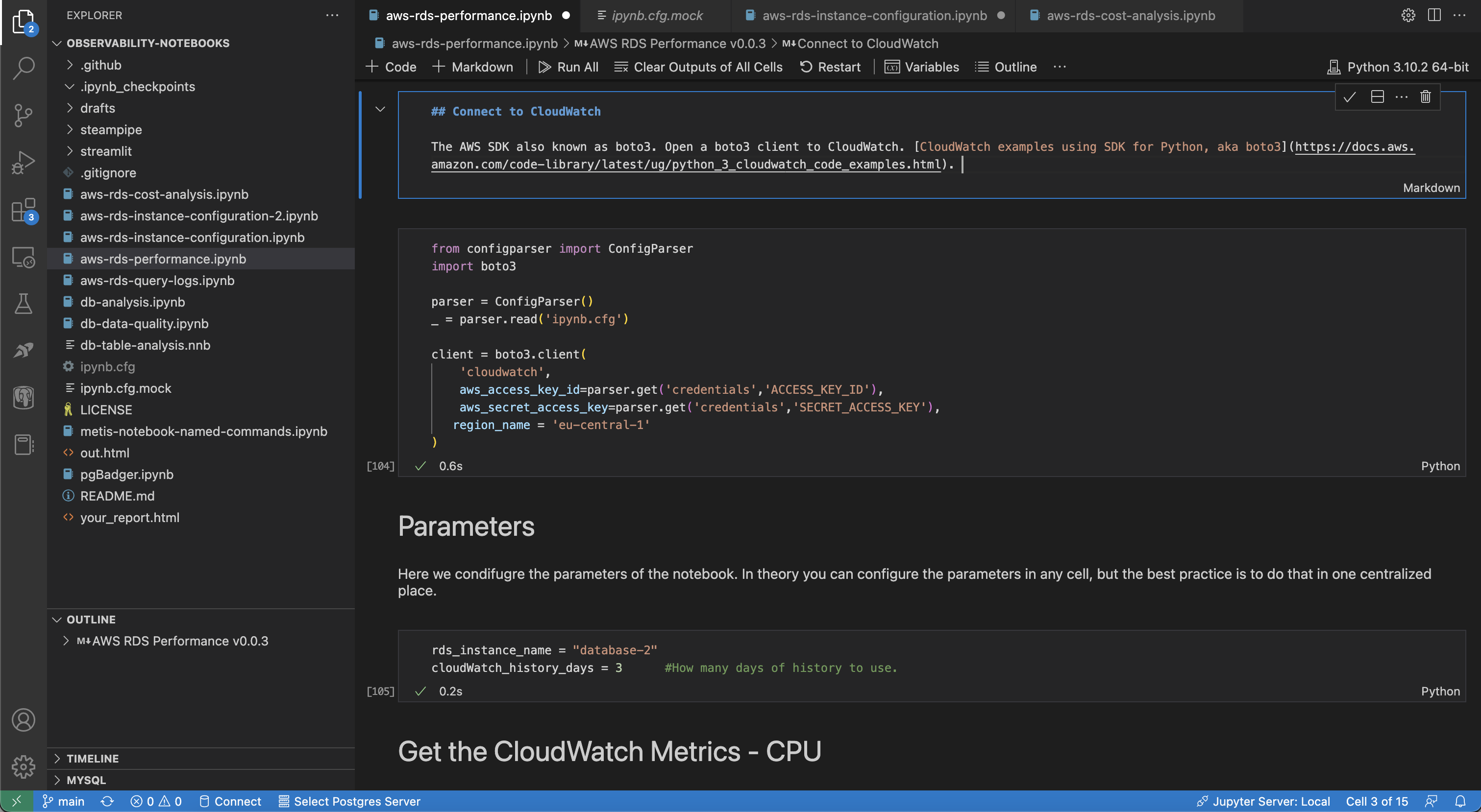
The AWS SDK is called boto3. The first step is configuring a client using AWS Credentials. It takes no more than 2 minutes to store the credentials in a configuration file similar to this one

from configparser import ConfigParser
import boto3

parser = ConfigParser()
_ = parser.read('ipynb.cfg')

client = boto3.client(
    'cloudwatch',
    aws_access_key_id=parser.get('credentials','ACCESS_KEY_ID'),
  aws_secret_access_key=parser.get('credentials','SECRET_ACCESS_KEY'),
   region_name = 'eu-central-1'
)

Now let's save the RDS name as a parameter:

rds_instance_name = "database-2"
cloudWatch_history_days = 3      #How many days of history to use.

And get the CPU utilization using the method GetMetricStatistics.

from datetime import datetime, timedelta, date
import pandas as pd

# TODO: replace the start and end date with now and now - 7. 
datapoints = client.get_metric_statistics(
    Namespace='AWS/RDS',
    MetricName='CPUUtilization',
     Dimensions=[
        {
            'Name': 'DBInstanceIdentifier',
            'Value': rds_instance_name
         },
     ],
    StartTime=datetime.today() - timedelta(days=cloudWatch_history_days),
    EndTime = datetime.today(),
    Period=3600,
    Statistics=['SampleCount','Average','Minimum','Maximum',
    ],
)

Storing the data as a Pandas DataFrame gives us endless possibilities to transform the data and visualize it as a table or chart.

from IPython.core.display import display, HTML
df_cpu = pd.DataFrame(datapoints['Datapoints'])

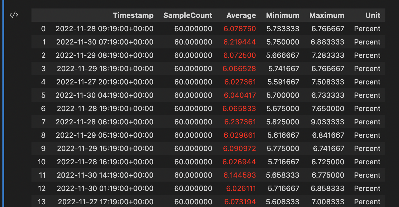
print(df_cpu)

The results set looks something like this

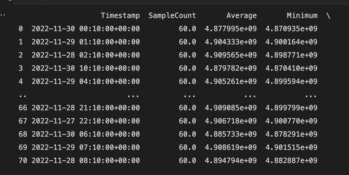
Not so user-friendly. So let's convert it to a chart or an HTML table with conditional formatting (color = red if condition is true).

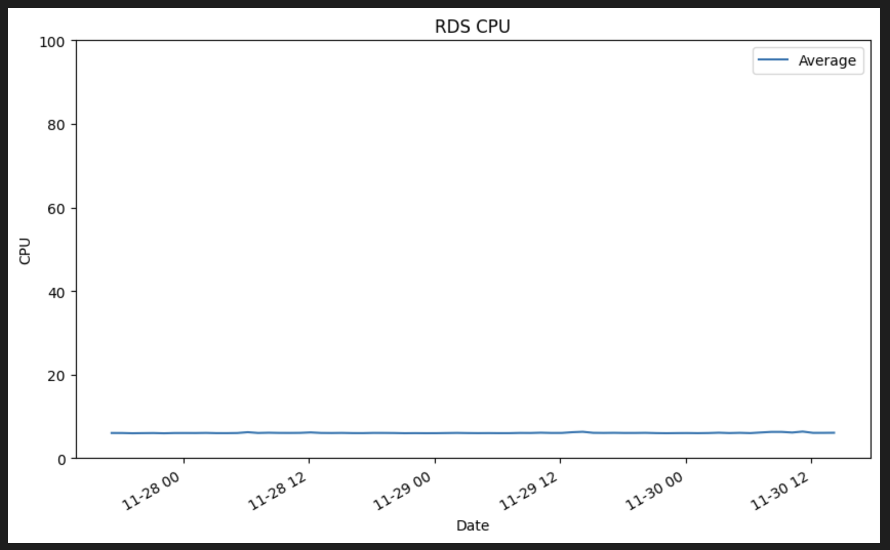
A chart:

mport matplotlib.pyplot as plt

df_cpu.plot(x='Timestamp', y='Average', kind='line')
# Trying to increase the size of the plot, as explained here: https://pythonguides.com/matplotlib-increase-plot-size/
plt.rcParams["figure.figsize"]=(10,6)
plt.ylim(0,100)
plt.title('RDS CPU')
plt.xlabel('Date')
plt.ylabel('CPU')
plt.show()

HTML Table

def color_negative_red(val):
    "Takes a scalar and returns a string with the css property `'color: red'` for negative strings, black otherwise."
    color = 'red' if int(val) >= 3 else 'white'
    return 'color: %s' % color
## You can either show the DataFrame as is (no formatting) or print it as HTML, highlighting values (conditional formatting) using the rule "color_negative_red"

display(HTML(df_cpu.style.applymap(color_negative_red, subset=pd.IndexSlice['Average']).to_html()))

The output looks similar to this

Shouldn't we use SteamPipe for this?

In the previous post I wrote about SteamPipe and how simple it is to get data from AWS CloudWatch and RDS instances using their SQL-based solution. So why her I used AWS SDK rather than SteamPipe?

Well, I started with SteamPipe and made good progress quickly. After all, it is just running SQL on a Postgres, a basic feature of Pandas. The data transformation is easy too, if you know SQL.

But, sometimes I needed to query AWS in a way that doesn't exist in SteamPipe. And once you learn how to use the AWS SDK for Python you can enjoy its flexibility and the ability to write back to AWS.

Conclusion

As a busy developer, who owns the DB, you need some kind of an Automated Investigation solution to quickly respond to events around performance, data quality, configuration, and schema migration. A DB in general and DB DevOps are complicated subjects, you should use Notebooks to automate parts of your work.